N-gram Networks • ParseR

ParseR combines functionality from the tidytext package and the tidygraph package to enable users to create network visualisations of common terms in a data set.

We’ll play through an example by creating a bi-gram network from a sample of the data set included in the ParseR package.

# Generate a sample
set.seed(1)
example <- ParseR::sprinklr_export %>%
  dplyr::slice_sample(n = 1000)

N.B. The function dplyr::slice_sample(n = 1000) is only used in this tutorial to speed up the analysis and workflow, a sample of 1000 should NOT be taken during project work. If you have any worries with the size of data or speed of analyses speak to one of the DS team.

Count the n-grams

Each post will be broken down into bi-grams (i.e. pairs of words) and the 25 most frequent bi-grams will be returned. The return counts will be equal to the number of times each bigram is seen in total across all mentions. If you would like to get the number of distinct posts each bigram is present in, add distinct = TRUE to the code.

counts <- example %>%
  ParseR::count_ngram(
    text_var = Message,
    n = 2,
    top_n = 25,
    clean_text = TRUE,
    remove_stops = TRUE
  )

As with all of the functions from our packages, you can access the documentation for each function by running the code ?count_ngram. This will allow you to see the arguments that can be fed to the function. In this case, the key arguments are text_var which requires the name of the column containing the text variable of interest, n which represents the number of terms to include in the n-gram (e.g. 2 produces a bi-gram), and top_n which determines the number of n-grams to include.

Note that counts is a list object:

class(counts)

## [1] "list"

It contains two objects:

“view”

A human-readable tibble with the most common n-grams.

counts %>%
  purrr::pluck("view")

## # A tibble: 25 × 3
##    word1       word2       ngram_freq
##    <chr>       <chr>            <int>
##  1 hispanic    heritage           503
##  2 heritage    month              253
##  3 heritage    celebration         39
##  4 celebrating hispanic            37
##  5 last        day                 33
##  6 national    hispanic            33
##  7 beto        orourke             32
##  8 bobby       beto                30
##  9 hispanic    caucus              30
## 10 lacks       hispanic            30
## # ℹ 15 more rows

“viz”

A tbl_graph object that can be used to produce a network visualisation.

counts %>%
  purrr::pluck("viz")

## # A tbl_graph: 27 nodes and 25 edges
## #
## # A directed acyclic simple graph with 3 components
## #
## # Node Data: 27 × 2 (active)
##    word        word_freq
##    <chr>           <int>
##  1 hispanic          638
##  2 heritage          531
##  3 month             275
##  4 day               107
##  5 celebration        96
##  6 us                 94
##  7 celebrating        81
##  8 last               67
##  9 new                58
## 10 celebrate          57
## # ℹ 17 more rows
## #
## # Edge Data: 25 × 3
##    from    to ngram_freq
##   <int> <int>      <int>
## 1     1     2        503
## 2     2     3        253
## 3     2     5         39
## # ℹ 22 more rows

Visualise the network

Now we can use the tbl_graph object we generated using count_ngrams() to produce a network visualisation by calling the viz_ngram function. An n-gram network is one of the most commonly produced visualisations at SHARE.

set.seed(123)
counts %>%
  purrr::pluck("viz") %>%
  ParseR::viz_ngram(emphasis = TRUE)

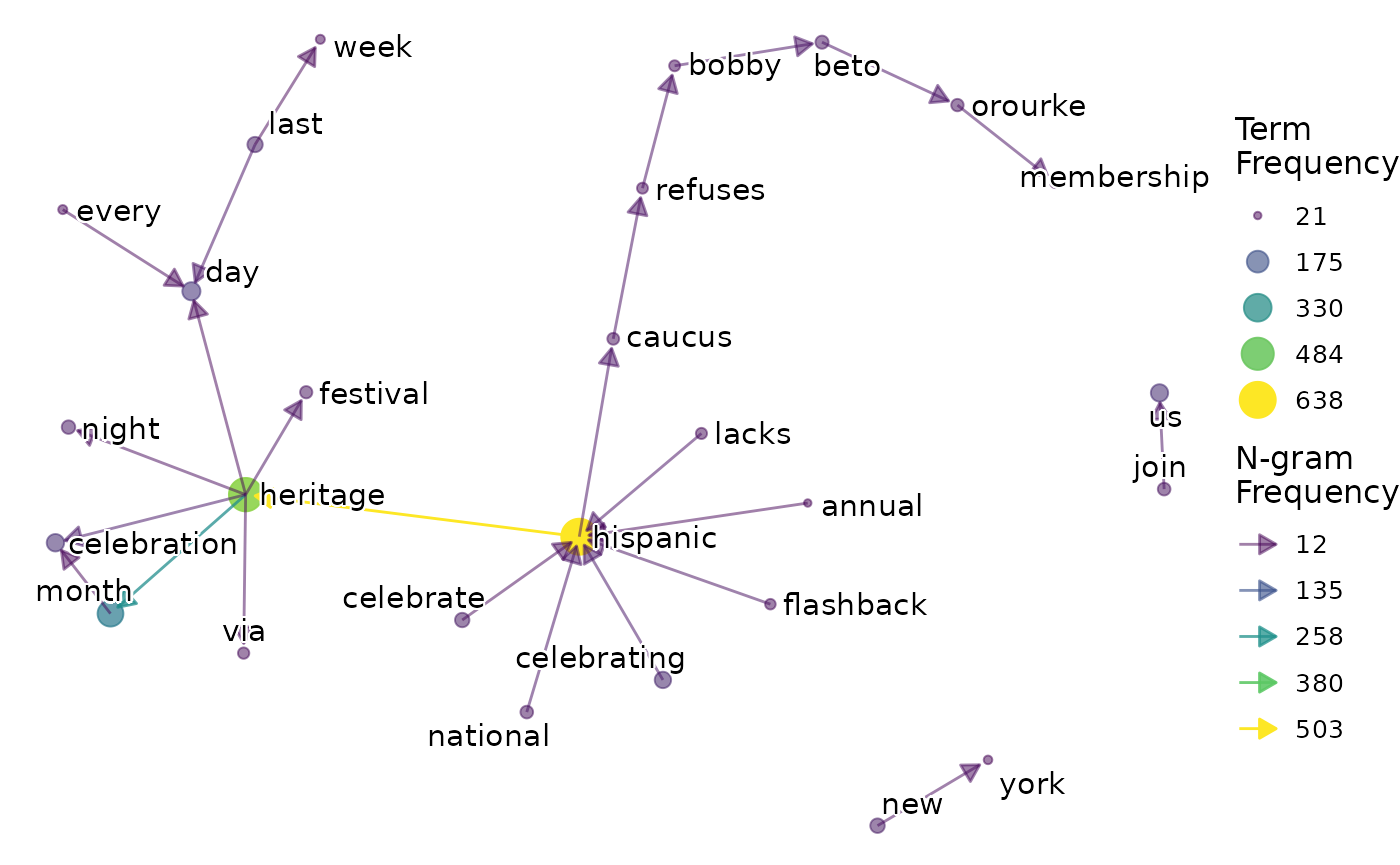
Note that visualising bi-grams in this way can be a useful way to also identify whether our cleaning steps have been sufficient for the task at hand:

If we see long chains of bi-grams consistently following one another (as in the case above with “caucus-refuses-bobby-beto”), this is often a good identifier for potential spam posts or posts that quote an identical phrase from an article, and are worth another check/ potential removal.
Bi-gram networks are very useful for identifying irrelevant terms that have snuck through our cleaning steps, such as URLs or homonyms (for example if the bi-gram is about Apple MacBooks, but there are bi-grams relating to Apple Crumble/Cooking Apple or similar).

As an additional tip relating to some bi-gram potential confusion. Sometimes a single term will appear in a bi-gram network, with seemingly no edge in or out of this node. In this case, the bi-gram phrase is a repeated term. This can be a ‘correct’ result: Say we are working with a manufacturer of tinned foods, a dataset may contain many phrases such as “this can can feed you and your family”. Therefore the bi-gram “can can” would appear in our network as a single node labelled “can”. However, such an outcome is much more likely to be the result of data cleaning where punctuation, numbers, or stop words have been removed and has led to two words appearing consecutively in the cleaned text variable, but not in the original text variable.

Term Context

We can also use the term_context function to plot the most frequent preceding/proceeding terms for the term of our choice, and gain a better understanding of how the term is used within the data.

latin_context <- example %>%
  ParseR::term_context(
    text_var = Message,
    term = "latin",
    preceding_n = 2,
    proceeding_n = 1,
    top_n = 10
  )

The outcome contains two objects:

“plot”

A graph object which displays the relationships between terms.

latin_context %>%
  purrr::pluck("plot")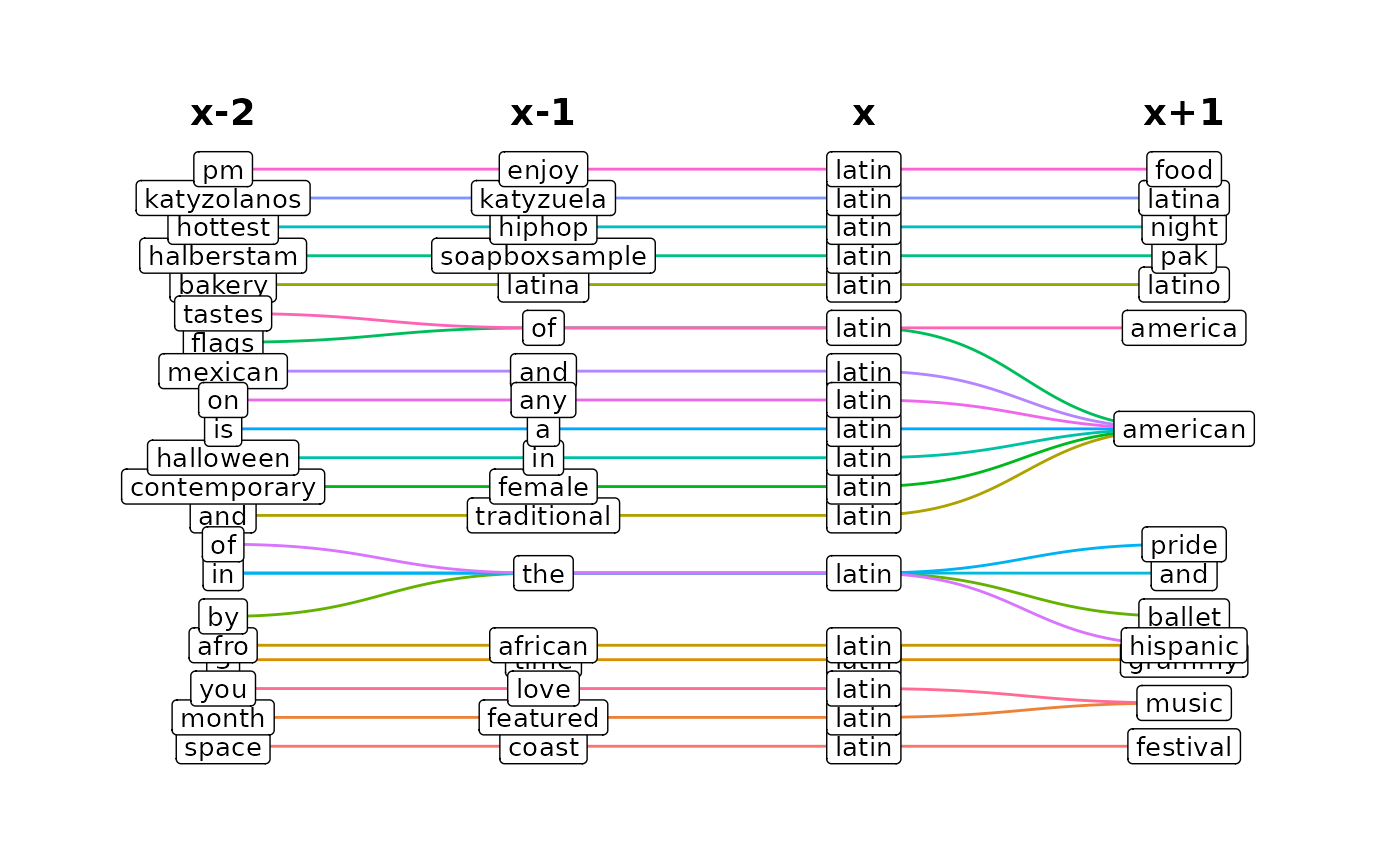

“frequencies”

A tibble which tells us how frequent the n-gram is in the data,

latin_context %>%
  purrr::pluck("frequencies")

## # A tibble: 22 × 5
##    `x-2`        `x-1`         x     `x+1`        n
##    <chr>        <chr>         <chr> <chr>    <int>
##  1 space        coast         latin festival     3
##  2 month        featured      latin music        2
##  3 3            time          latin grammy       1
##  4 afro         african       latin hispanic     1
##  5 and          traditional   latin american     1
##  6 bakery       latina        latin latino       1
##  7 by           the           latin ballet       1
##  8 contemporary female        latin american     1
##  9 flags        of            latin american     1
## 10 halberstam   soapboxsample latin pak          1
## # ℹ 12 more rows

Extracting n-gram exemplar posts

A new update to ParseR gives us the opportunity to extract exemplar posts for our ngrams. We receive a dataframe with the columns: [1] “ngram_n” “ngrams” “message” “permalink” “sentiment” “date” “author”
[8] “platform”

Note: some variable names may change, and they are lower-cased.

exemplars <- ParseR::ngram_exemplars(example, text_var = Message, url_var = Permalink, sentiment_var = Sentiment, date_var = CreatedTime, author_var = SenderScreenName, platform_var = SocialNetwork)

We could turn our exemplars into a nice data table with clickable links using the {DT} package and a {LimpiaR} function:

exemplars %>%
  LimpiaR::limpiar_link_click(permalink) %>%
  DT::datatable(escape = FALSE, filter = "top", options = list(scrollX = TRUE))